Block convoluiton using skew transform (overlap-add method)

Contents

Overlap-add method

function []=overlapaddqdft_demo()

% Classic overlap-add method is using FFT size of 2N, where N is block size [1].
% Proposed method is using skew transform of size N for computation reduction [2].
% Convolution mod(x^N-j) is used for each block, and the skew transform is
% an eigen transform of this skew convolution.
% It is easy to see that multiplication of two polynomials y(z)=x(z)*h(z) (mod (x^N-j)),
% where x(z)=x(0)+x(1)*z+x(2)*z^2+..+x(N-1)*z^(N-1) is an input signal,
% and h(z)=h(0)+h(1)*z+h(2)*z^2+..+h(N-1)*z^(N-1) is impulse response of a filter,
% will give result of block convolution
% if output is read as Y=[Re(y(0))... Re(y(N-1)), Im(y(0))... Im(y(N-1))].

Init

N=32;   % block size

x=randn(1,5*N);     % input signal
h=randn(1,N);       % filter impulse response

% y=fftfilt(h,x);   % true result

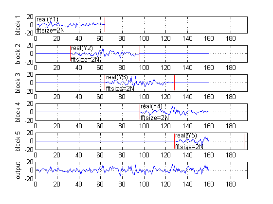
Classic overlap-add method (FFT size = 2*N)

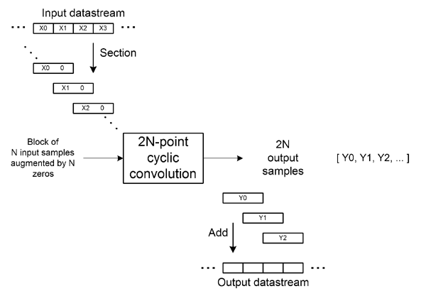
hs=fft(h',2*N);                 % filter spectral response
xn=reshape(x,N,[]);
xn=[xn; zeros(size(xn))];
xs=fft(xn);                     % block spectrum of input signal (FFT size = 2*N)
ys=bsxfun(@times,hs,xs);        % spectral domain multiplication
y1=real(ifft(ys));              % block convolution result
y2=y1(1:N,:)+[zeros(N,1) y1((1:N)+N,1:end-1)];      % overlap-add block combination
ycl=reshape(y2,[],1);

% block-wise graph
figure(2)
plot_blockwise_classic(y1,N,length(x))

subplot(size(y1,2)+1,1,size(y1,2)+1);
plot(ycl)
axis([0 round(length(x)+N*1.1) -20 20]);
grid on
ylabel(['output']);

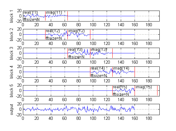
Proposed overlap-add method (FFT size = N)

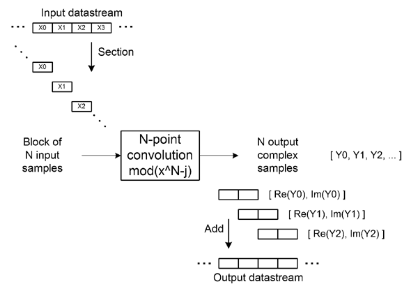
w=exp(1i*pi/2/N*(0:N-1)');              % diagonal elements for qDFT
hs=fft(w.*h');

xn=reshape(x,N,[]);
x1=bsxfun(@times,w,xn);                 % pre-multiplication by diagonal twiddle factors
s1=fft(x1);                             % block spectrum of input signal (qDFT size = N)
s2=bsxfun(@times,hs,s1);                % spectral domain multiplication
y1=bsxfun(@times,conj(w),ifft(s2));     % inverse skew transform, block convolution result
y2=real(y1)+[zeros(N,1) imag(y1(:,1:end-1))];      % overlap-add block combination (output is read as Y=[Re(y(0))... Re(y(N-1)), Im(y(0))... Im(y(N-1))])
ypr=reshape(y2,1,[]);

% block-wise graph
figure(1)
% title('Proposed qDFT based method');
plot_blockwise_propose(y1,N,length(x))

% plot resulting output
subplot(size(y1,2)+1,1,size(y1,2)+1);
plot(ypr)
axis([0 round(length(x)+N*1.1) -20 20]);
grid on
ylabel(['output']);

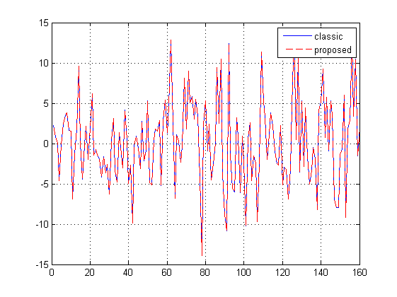
Compare results

figure(3)
plot(ycl)
hold on
plot(ypr,'--r');
hold off
grid on
legend('classic','proposed')

References

[1] Blahut, R.E.: Fast Algorithms for Signal Processing. Cambridge University Press (2010). (p. 198)

[2] Jung Gap Kuk, Seyun Kim, and Nam Ik Cho, "A New Overlap Save Algorithm for Fast Block Convolution and Its Implementation Using FFT," Journal of Signal Processing Systems(Online), Feb 2010.

function []=plot_blockwise_classic(y1,N,lenx)
for i=1:size(y1,2),
    y9=zeros(size(y1));
    y9(:,i)=y1(:,i);
    y9=y9(1:N,:)+[zeros(N,1) y9((1:N)+N,1:end-1)];
    y9=reshape(real(y9),1,[]);
    subplot(size(y1,2)+1,1,i);
    plot(y9)
    hold on
    a=17;
    plot([0 0]+(i-1)*N,[-a a],'r');
    plot([0 0]+(i-1+2)*N,[-a a],'r');
    text(1+(i-1)*N,-a*0.8,'fftsize=2N');
    text(1+(i-1)*N,a*0.8,['real(Y' num2str(i) ')']);
    hold off
    axis([0 round(lenx+N*1.1) -20 20]);
    grid on
    ylabel(['block ' num2str(i)]);
end

function []=plot_blockwise_propose(y1,N,lenx)
for i=1:size(y1,2),
    y9=zeros(size(y1));
    y9(:,i)=y1(:,i);
    y9(:,2:end)=real(y9(:,2:end))+imag(y9(:,1:end-1));
    y9=reshape(real(y9),1,[]);
    subplot(size(y1,2)+1,1,i);
    plot(y9)
    hold on
    a=17;
    plot([0 0]+(i-1)*N,[-a a],'r');
    plot([0 0]+(i-1+1)*N,[-a a],'r');
    plot([0 0]+(i-1+2)*N,[-a a],'r');
    text(1+(i-1)*N,-a*0.8,'fftsize=N');
    text(1+(i-1)*N,a*0.8,['real(Y' num2str(i) ')']);
    text(1+(i-1+1)*N,a*0.8,['imag(Y' num2str(i) ')']);
    hold off
    axis([0 round(lenx+N*1.1) -20 20]);
    grid on
    ylabel(['block ' num2str(i)]);
end

Published with MATLAB® R2014a