EMQF filters
EMQF filters (Elliptic filters with maximal Q-factor) are special case of elliptic filters. EMQF filters have equal ripples in passband and in stopband as well. They require three design parameters (ripple in stopband, cut-off frequency for passband, and cut-off frequency for stopband). Next we will present several applications of these filters
Contents
1. Allpass realization
Not only elliptic filters but every odd order elliptic and butterworth filters can be realized as a parallel connection of two alllpasses using 'tf2ca' function.
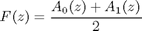
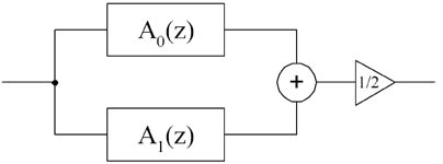
Fig.1. Realization of IIR filter as a coupled allpass filter connection.
Let us design an elliptic low-pass filter
%[num0, den0]=ellip(5,2,40,0.3)                             % transfer function of elliptic filter
[num0, den0]=ellip(7,2,40,0.3)                             % transfer function of elliptic filter
fvtool(num0,den0);
num0 =
    0.0237   -0.0386    0.0604   -0.0148   -0.0148    0.0604   -0.0386    0.0237
den0 =
    1.0000   -4.4713   10.0742  -14.0199   12.9236   -7.8394    2.9149   -0.5207
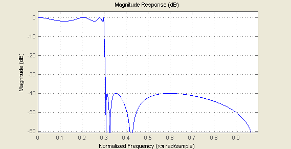
Fig.2. Frequency response of original filter
Now we will represent it as a coupled-allpass structure
[d0,d1]=tf2ca(num0,den0); p0=fliplr(d0); p1=fliplr(d1);     % transfer function of filters in coupled-allpass scheme
p0,d0,p1,d1
p0 =
    0.7457   -2.2130    3.3183   -2.5163    1.0000
d0 =
    1.0000   -2.5163    3.3183   -2.2130    0.7457
p1 =
   -0.6983    1.8366   -1.9550    1.0000
d1 =
    1.0000   -1.9550    1.8366   -0.6983
And plot frequency response of this structure
x=[1 zeros(1,1000)];
y=(filter(p0,d0,x)+filter(p1,d1,x))/2;                      % impulse response of coupled-allpass scheme

fvtool(y,1);

Fig. 3. Frequency response of coupled all-pass structure
Comparison of Fig.2 and Fig.3 shows that transfer functions of both classic and coupled-allpass realizations are identical.
By using 'tf2sos' function we can realize this filter by means of three biquads and one first order IIR.
sos0=tf2sos(p0,d0)
sos1=tf2sos(p1,d1)
sos0 =
    0.7457   -1.3291    0.9884    1.0000   -1.3447    0.7545
    1.0000   -1.1854    1.0118    1.0000   -1.1716    0.9884
sos1 =
   -0.6983    0.9338         0    1.0000   -0.7478         0
    1.0000   -1.2928    1.0709    1.0000   -1.2072    0.9338
Fig.4. Realization of filter from example by means of allpass elements.
Note, that original filter order is equal to the sum of filter orders in coupled-allpass structure. It allows realizing elliptic filter with less number of coefficients. By using structures presented in [1] we can achieve less computational complexity.
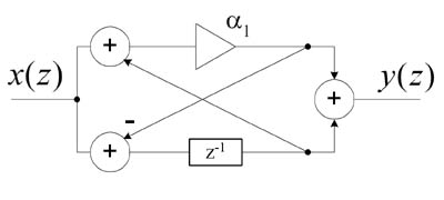
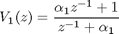
Fig. 5. Realization of first order IIR allpass filter.
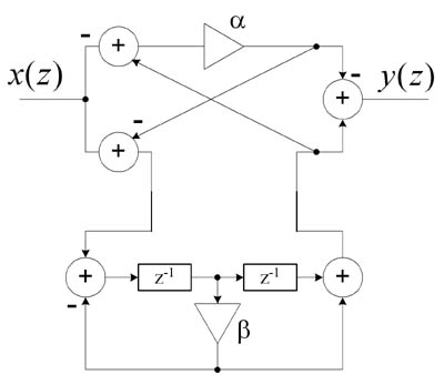
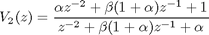
Fig. 6. Realization of second order IIR allpass filter.
Coefficients for these structures are defined as follows
2. EMQF filter design
Example below demonstrates design of EMQF lowpass filter [2] by means of 'ellip_du' function. This function directly computes coefficients of all-pass filters.
'p0' and 'd0' are numerator and denominator of all-pass A0(z)
'p1' and 'd1' are numerator and denominator of all-pass A1(z)
F3db=0.15;
df=0.04;
[p1,d1,p0,d0]=apellip_du(9,F3db-df,F3db+df)
fvtool((filter(p0,d0,x)+filter(p1,d1,x))/2);
p1 =
   -0.1132    0.7293   -1.9125    2.8733   -2.3121    1.0000
d1 =
    1.0000   -2.3121    2.8733   -1.9125    0.7293   -0.1132
p0 =
    0.1198   -0.6397    1.5268   -1.7080    1.0000
d0 =
    1.0000   -1.7080    1.5268   -0.6397    0.1198
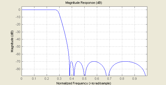
Fig.7. Frequency response of EMQF low-pass filter
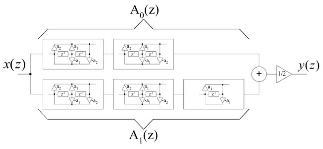
Fig. 8. Coupled-allpass realization of EMQF filter.
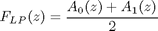
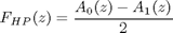
3. LP+HP complementary pair of filters
If low-pass filter is represented as a sum of two all-passes, complementary high-pass filter is represented as a difference of them.
fvtool((filter(p0,d0,x)+filter(p1,d1,x))/2,1,(filter(p0,d0,x)-filter(p1,d1,x))/2,1);
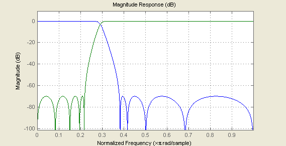
Fig. 9. Complementary pair of filters
Sum of these two complementary filters is allpass filter (magnitude response is flat).

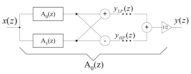
Fig. 10. Splitting and combining subband by means of EMQF filters.
So we have two good points:
1. Two filters are realized by the cost of one filter plus one addition operation.
2. We can split signal into subbands and then easily combine them again without magnitude distortions.
4. Decimation and interpolation based on EMQF filters
Consider case of decimation/interpolation by two. For this case we need a halfband filter as a decimation filter. We will use EMQF filter for this purpose.
F3db=0.25;
df=0.02;
[p1,d1,p0,d0]=apellip_du(9,F3db-df,F3db+df)
fvtool((filter(p0,d0,x)+filter(p1,d1,x))/2);
p1 =
   -0.0000    0.3855   -0.0000    1.3313   -0.0000    1.0000
d1 =
    1.0000   -0.0000    1.3313   -0.0000    0.3855   -0.0000
p0 =
    0.0947   -0.0000    0.8335   -0.0000    1.0000
d0 =
    1.0000   -0.0000    0.8335   -0.0000    0.0947
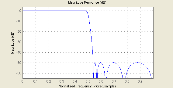
Fig. 11. Frequency response of Halfband lowpass filter
Note that half of coefficients in all-pass realization are equal to zero, and halfband decimation EMQF filter can be represented in the form of two polyphase components

where
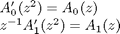
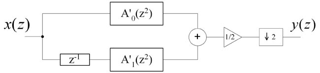
Fig. 12. Realization of decimation filter as coupled-allpass.
So, similar to FIR filter case, decimation can be realized using polyphase filtering. Filter A1(z) filters even samples of input signal, and filter A0(z) filters odd samples of input signal.
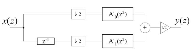
Fig. 13. Polyphase realization of decimation filter.
5. Hilbert transform pair IIR filters
Halfband filter designed in previous part can be used for making Hilbert transform IIR pair. This approach is based on shifting frequency response of halfband filter on pi/2 (half of Nyquist frequency), i.e in previous equation 'z' should be multiplied by exp(-j*pi/2) [3].

p0=p0.*(j.^((0:length(p0)-1)))
d0=d0.*(j.^((0:length(d0)-1)))
p1=p1.*(j.^((0:length(p1)-1)-1))
d1=d1.*(j.^((0:length(d1)-1)))
y0=filter(p0,d0,x)/2;
y1=filter(p1,d1,x)/2;
fvtool(y0+j*y1);
p0 =
  Columns 1 through 4
   0.0947                  0 - 0.0000i  -0.8335                  0 + 0.0000i
  Column 5
   1.0000
d0 =
  Columns 1 through 4
   1.0000                  0 - 0.0000i  -0.8335                  0 + 0.0000i
  Column 5
   0.0947
p1 =
  Columns 1 through 4
        0 + 0.0000i   0.3855                  0 - 0.0000i  -1.3313
  Columns 5 through 6
        0 + 0.0000i   1.0000
d1 =
  Columns 1 through 4
   1.0000                  0 - 0.0000i  -1.3313                  0 + 0.0000i
  Columns 5 through 6
   0.3855                  0 - 0.0000i
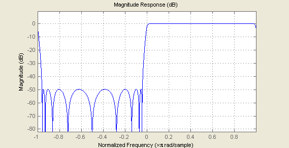
Fig. 14. Magnitude spectrum of analytic signal
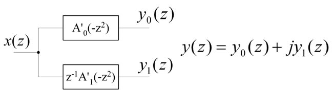
Fig. 15. Hilbert IIR pair based on EMQF halfband filter.
Complex signal y0+j*y1 has non-zero spectrum only at positive frequencies. Hence, y0 and y1 are Hilbert pair signals. Note that IIR filters based on EMQF filters have two times less computational complexity due to the fact that every second coefficient in transfer function is zero.
6. Multiplierless realization of EMQF filters
Example below shows designing multiplierless EMQF filter with the same parameters as in chapter 3. As shown in [4], coefficient 'beta' is dependent only from cut-off frequency F3db. Coefficients 'alpha' and 'alpha1' are coefficients in special realizations of all-pass biquads (see Fig.1).
[alpha,beta,alpha1]=ellipEMQF_nomult(9, F3db-df,F3db+df, 1, 42)
[num,den]=(emqf_co2tf(alpha,beta,alpha1))
fvtool(num,den);
Calculating 'alpha'...
Calculating maximal 'beta'...
Optimization terminated: norm of relative change in X is less
 than max(options.TolX^2,eps) and  sum-of-squares of function
 values is less than sqrt(options.TolFun).
Calculating 'beta's...
Calculating 'alpha1'...
alpha =
     0
beta =
    0.1563    0.4688    0.7383    0.9219
alpha1 =
   -0.0020
num =
  Columns 1 through 9
    0.0572    0.2160    0.5257    0.8875    1.1446    1.1446    0.8875    0.5257    0.2160
  Column 10
    0.0572
den =
  Columns 1 through 9
    1.0000   -0.0020    2.2852   -0.0045    1.7914   -0.0036    0.5470   -0.0011    0.0498
  Column 10
   -0.0001
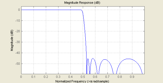
Fig. 16. Frequency response of muliplierless EMQF lowpass filter
Comparison of figures 5 and 7 shows that in multiplierless implementation we loose about 4dB only.
Note, that function 'ellipEMQF_nomult' considers 16-bit precision for coefficients and 4 non-zero numbers in {-1,1} set inbetween of 16 bits.
alpha_bin =[char(ones(1,floor((1-sign(alpha))/2))*'-')    '.' dec2bin(round (abs(alpha)*2^16),16 )]
beta1_bin =[char(ones(1,floor((1-sign(beta(1)))/2))*'-')  '.' dec2bin(round (abs(beta(1))*2^16),16 )]
beta2_bin =[char(ones(1,floor((1-sign(beta(2)))/2))*'-')  '.' dec2bin(round (abs(beta(2))*2^16),16 )]
beta3_bin =[char(ones(1,floor((1-sign(beta(3)))/2))*'-')  '.' dec2bin(round (abs(beta(3))*2^16),16 )]
beta4_bin =[char(ones(1,floor((1-sign(beta(4)))/2))*'-')  '.' dec2bin(round (abs(beta(4))*2^16),16 )]
alpha1_bin=[char(ones(1,floor((1-sign(alpha1))/2))*'-')   '.' dec2bin(round (abs(alpha1)*2^16),16 )]
alpha_bin =
.0000000000000000
beta1_bin =
.0010100000000000
beta2_bin =
.0111100000000000
beta3_bin =
.1011110100000000
beta4_bin =
.1110110000000000
alpha1_bin =
-.0000000010000010
You can check that each multiplier can be realized by means of no more than 4 addition/subtraction operations.
Actually, alpha1 is zero for halfband filter (check it with 'ellip_du' function). This small non-zero value arises due to error of numerical optimization.
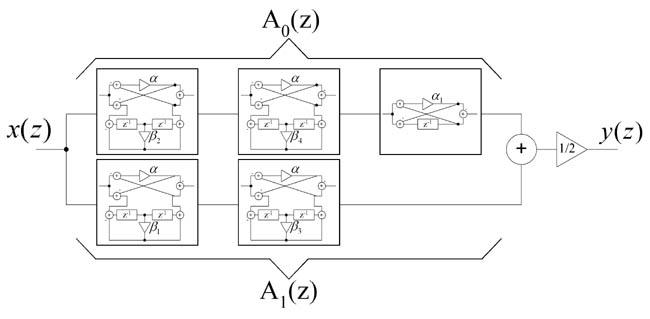
Fig. 17. Multiplierless realization of EMQF filter.
References
[1] Ansari, R., and Liu, B. (1985, February). A class of low-noise computationally efficient recursive digital filters with applications to sampling rate alternations. IEEE Transactions on Acoustics, Speech, and Signal Processing, Vol. 33, pp. 90-97.
[2] Lj. D. Milic, M. D. Lutovac, Efficient Algorithm for the Design of High-Speed Elliptic IIR Filters, Int. Journal of Electronics and Communications, AEU, Vol. 57, No. 4, 2003, pp. 255-262.
[3] M. Lutovac, Lj. Milic, Design of multiplierless elliptic IIR halfband filters and Hilbert transformers, 9th European Signal Processing Conference EUSIPCO'98, Rodos, Greece, Sep. 1998, pp. 291-294.
[4] Lj. D. Milic, M. D. Lutovac, Design of multiplierless elliptic IIR filters with a small quantization error, IEEE Trans. Signal Processing, Vol. 47, no. 2, Feb. 1999, pp. 469-479.