Relations between DCTV and DSTV
Contents
- Definitions
- DCTV matrix definition
- DCTV in terms of Tschebyshev polynomials
- DSTV matrix definition
- DSTV in terms of Tschebyshev polynomials
- Finding relations
- Check expression of DCTV through DSTV
- Check expression of DSTV through DCTV
- Check computation of DCTV transform
- Check computation of DSTV transform
- Reference
Definitions
Transform matrix is defined for operating on column-vectors y=T*x, where y, x are column-vectors, T is transform matrix
DCTV matrix definition
N1=9; N=N1;
k=0:N1-1;  l=0:N1-1;
DCT5=cos(pi/(N-1/2)*k'*l)       % display DCTV matrix
DCT5 =
  Columns 1 through 7
    1.0000    1.0000    1.0000    1.0000    1.0000    1.0000    1.0000
    1.0000    0.9325    0.7390    0.4457    0.0923   -0.2737   -0.6026
    1.0000    0.7390    0.0923   -0.6026   -0.9830   -0.8502   -0.2737
    1.0000    0.4457   -0.6026   -0.9830   -0.2737    0.7390    0.9325
    1.0000    0.0923   -0.9830   -0.2737    0.9325    0.4457   -0.8502
    1.0000   -0.2737   -0.8502    0.7390    0.4457   -0.9830    0.0923
    1.0000   -0.6026   -0.2737    0.9325   -0.8502    0.0923    0.7390
    1.0000   -0.8502    0.4457    0.0923   -0.6026    0.9325   -0.9830
    1.0000   -0.9830    0.9325   -0.8502    0.7390   -0.6026    0.4457
  Columns 8 through 9
    1.0000    1.0000
   -0.8502   -0.9830
    0.4457    0.9325
    0.0923   -0.8502
   -0.6026    0.7390
    0.9325   -0.6026
   -0.9830    0.4457
    0.7390   -0.2737
   -0.2737    0.0923
DCTV in terms of Tschebyshev polynomials
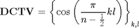
The DCTV matrix can be expressed in terms of Tschebyshev polynomials [1]
![$${\mathbf {DCTV}} = \left[ {T_l \left( {\alpha _k } \right)} \right]_{k,l} $$](DCTV_DSTV_eq28569.png)
where
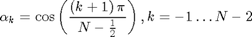
are roots of polynomial
alpha=sort([roots(TschebyshevW(N-1)); 1],'descend');
DCT5t=zeros(N1);
for l=0:N1-1,
    DCT5t(:,l+1)=polyval(TschebyshevT(l),alpha)';
end
Da5=diag(cos(0*pi/(N-1/2)*k));
DCT5t=Da5*DCT5t                    % display DCTV matrix

% compare DCT5 and DCT5t matrices (show that both definitions above are equivalent)
max(max(abs(DCT5-DCT5t)))
DCT5t =
  Columns 1 through 7
    1.0000    1.0000    1.0000    1.0000    1.0000    1.0000    1.0000
    1.0000    0.9325    0.7390    0.4457    0.0923   -0.2737   -0.6026
    1.0000    0.7390    0.0923   -0.6026   -0.9830   -0.8502   -0.2737
    1.0000    0.4457   -0.6026   -0.9830   -0.2737    0.7390    0.9325
    1.0000    0.0923   -0.9830   -0.2737    0.9325    0.4457   -0.8502
    1.0000   -0.2737   -0.8502    0.7390    0.4457   -0.9830    0.0923
    1.0000   -0.6026   -0.2737    0.9325   -0.8502    0.0923    0.7390
    1.0000   -0.8502    0.4457    0.0923   -0.6026    0.9325   -0.9830
    1.0000   -0.9830    0.9325   -0.8502    0.7390   -0.6026    0.4457
  Columns 8 through 9
    1.0000    1.0000
   -0.8502   -0.9830
    0.4457    0.9325
    0.0923   -0.8502
   -0.6026    0.7390
    0.9325   -0.6026
   -0.9830    0.4457
    0.7390   -0.2737
   -0.2737    0.0923
ans =
   2.5746e-13
DSTV matrix definition
N2=8; N=N2;
k=0:N2-1;  l=0:N2-1;
DST5=sin(pi/(N+1/2)*(k+1)'*(l+1))       % display DCTV matrix
DST5 =
  Columns 1 through 7
    0.3612    0.6737    0.8952    0.9957    0.9618    0.7980    0.5264
    0.6737    0.9957    0.7980    0.1837   -0.5264   -0.9618   -0.8952
    0.8952    0.7980   -0.1837   -0.9618   -0.6737    0.3612    0.9957
    0.9957    0.1837   -0.9618   -0.3612    0.8952    0.5264   -0.7980
    0.9618   -0.5264   -0.6737    0.8952    0.1837   -0.9957    0.3612
    0.7980   -0.9618    0.3612    0.5264   -0.9957    0.6737    0.1837
    0.5264   -0.8952    0.9957   -0.7980    0.3612    0.1837   -0.6737
    0.1837   -0.3612    0.5264   -0.6737    0.7980   -0.8952    0.9618
  Column 8
    0.1837
   -0.3612
    0.5264
   -0.6737
    0.7980
   -0.8952
    0.9618
   -0.9957
DSTV in terms of Tschebyshev polynomials
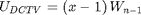
The DSTV matrix can be expressed in terms of Tschebyshev polynomials [1]
![$$
{\mathbf{DSTV}}\mathrm{{=}}{\mathbf{D}}_{DSTV}\mathrm{\cdot}{\mathrm{\left[{{U}_{l}\left({{\mathit{\beta}}_{k}}\right)}\right]}}_{k\mathrm{,}l}
$$](DCTV_DSTV_eq54094.png)
where
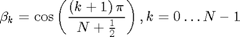
are roots of polynomial

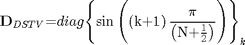
beta=sort([roots(TschebyshevW(N))],'descend');
DST5t=zeros(N);
for l=0:N2-1,
    DST5t(:,l+1)=polyval(TschebyshevU(l),beta)';
end
Db5=diag(sin(pi/(N+1/2)*(k+1)));
DST5t=Db5*DST5t                    % display DCTV matrix

% compare DST5 and DST5t matrices (show that both definitions above are equivalent)
max(max(abs(DST5-DST5t)))
DST5t =
  Columns 1 through 7
    0.3612    0.6737    0.8952    0.9957    0.9618    0.7980    0.5264
    0.6737    0.9957    0.7980    0.1837   -0.5264   -0.9618   -0.8952
    0.8952    0.7980   -0.1837   -0.9618   -0.6737    0.3612    0.9957
    0.9957    0.1837   -0.9618   -0.3612    0.8952    0.5264   -0.7980
    0.9618   -0.5264   -0.6737    0.8952    0.1837   -0.9957    0.3612
    0.7980   -0.9618    0.3612    0.5264   -0.9957    0.6737    0.1837
    0.5264   -0.8952    0.9957   -0.7980    0.3612    0.1837   -0.6737
    0.1837   -0.3612    0.5264   -0.6737    0.7980   -0.8952    0.9618
  Column 8
    0.1837
   -0.3612
    0.5264
   -0.6737
    0.7980
   -0.8952
    0.9618
   -0.9957
ans =
   1.4100e-13
Finding relations
Because there exist relation

and
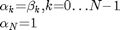
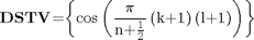
we can express DCTV through DSTV
![$$ \begin{array}{l}
{{\mathbf{DCTV}}\mathrm{{=}}{\left[{{T}_{l}\left({{\mathit{\alpha}}_{k}}\right)}\right]}_{k\mathrm{,}l}\mathrm{{=}}{\left[{\begin{array}{cc}{1}&{}\\{}&{{U}_{l}\left({{\mathit{\beta}}_{k}}\right)}\end{array}}\right]}_{k\mathrm{,}l}\mathit{\cdot}{\mathbf{B}}\mathrm{{=}}\mathrm{\left[{\begin{array}{cc}{1}&{}\\{}&{{\left({{\mathbf{D}}_{DSTV}}\right)}^{{-}{1}}\mathit{\cdot}{\mathbf{D}}_{DSTV}\mathit{\cdot}{\left[{{U}_{l}\left({{\mathit{\beta}}_{k}}\right)}\right]}_{k,l}}\end{array}}\right]}\mathit{\cdot}{\mathbf{B}}\mathrm{{=}}}\\
{\mathrm{{=}}\mathrm{\left[{\begin{array}{cc}{1}&{}\\{}&{{\left({{\mathbf{D}}_{DSTV}}\right)}^{{-}{1}}\cdot{\mathbf{DSTV}}}\end{array}}\right]}\mathrm{\cdot}{\mathbf{B}}}
\end{array}$$](DCTV_DSTV_eq40670.png)
where
![$${\mathbf{B}}\mathrm{{=}}\frac{1}{2}\left[{\begin{array}{cccccc}{2}&{2}&{2}&{\mathrm{\cdots}}&{2}&{2}\\{2}&{}&{\mathrm{{-}}{1}}&{}&{}&{}\\{}&{1}&{}&{\mathrm{\ddots}}&{}&{}\\{}&{}&{1}&{\mathrm{\ddots}}&{\mathrm{{-}}{1}}&{}\\{}&{}&{}&{\mathrm{\ddots}}&{}&{\mathrm{{-}}{1}}\\{}&{}&{}&{}&{1}&{\mathrm{{-}}{1}}\end{array}}\right]$$](DCTV_DSTV_eq97944.png)
B=toeplitz([0.5 zeros(1,N-1)]',[0.5           0        -0.5 zeros(1,N-length([0.5           0        -0.5]))]);
B(1,1)=1;
B=[B [0; B(1:end-1,end)]];
B(8,9)=-0.5;
B=[ones(1,size(B,2)); B];
Check expression of DCTV through DSTV
![$$
{\mathbf{DCTV}}\mathrm{{=}}\mathrm{\left[{\begin{array}{cc}{1}&{}\\{}&{{\left({{\mathbf{D}}_{DSTV}}\right)}^{{-}{1}}\cdot{\mathbf{DSTV}}}\end{array}}\right]}\mathrm{\cdot}{\mathbf{B}}
$$](DCTV_DSTV_eq56300.png)
DCT5a=Da5*blkdiag(1,inv(Db5)*DST5)*B
% compare DCT5 and DCT5a matrices (show correctness of representation of DCTV through DSTV)
max(max(abs(DCT5-DCT5a)))
DCT5a =
  Columns 1 through 7
    1.0000    1.0000    1.0000    1.0000    1.0000    1.0000    1.0000
    1.0000    0.9325    0.7390    0.4457    0.0923   -0.2737   -0.6026
    1.0000    0.7390    0.0923   -0.6026   -0.9830   -0.8502   -0.2737
    1.0000    0.4457   -0.6026   -0.9830   -0.2737    0.7390    0.9325
    1.0000    0.0923   -0.9830   -0.2737    0.9325    0.4457   -0.8502
    1.0000   -0.2737   -0.8502    0.7390    0.4457   -0.9830    0.0923
    1.0000   -0.6026   -0.2737    0.9325   -0.8502    0.0923    0.7390
    1.0000   -0.8502    0.4457    0.0923   -0.6026    0.9325   -0.9830
    1.0000   -0.9830    0.9325   -0.8502    0.7390   -0.6026    0.4457
  Columns 8 through 9
    1.0000    1.0000
   -0.8502   -0.9830
    0.4457    0.9325
    0.0923   -0.8502
   -0.6026    0.7390
    0.9325   -0.6026
   -0.9830    0.4457
    0.7390   -0.2737
   -0.2737    0.0923
ans =
   1.9429e-15
Check expression of DSTV through DCTV
![$$\left[{\begin{array}{cc}{1}&{}\\{}&{\mathbf{DSTV}}\end{array}}\right]\mathrm{{=}}\mathrm{\left[{\begin{array}{cc}{1}&{}\\{}&{{\mathbf{D}}_{DSTV}}\end{array}}\right]}\mathrm{\cdot}{\mathbf{DCTV}}\mathrm{\cdot}{\mathbf{B}}^{\mathrm{{-}}{1}}$$](DCTV_DSTV_eq69798.png)
DST5a=blkdiag(1,Db5)*inv(Da5)*DCT5*inv(B);
DST5a=DST5a(2:end,2:end)
% compare DST5 and DST5a matrices (show correctness of representation of DSTV through DCTV)
max(max(abs(DST5-DST5a)))
DST5a =
  Columns 1 through 7
    0.3612    0.6737    0.8952    0.9957    0.9618    0.7980    0.5264
    0.6737    0.9957    0.7980    0.1837   -0.5264   -0.9618   -0.8952
    0.8952    0.7980   -0.1837   -0.9618   -0.6737    0.3612    0.9957
    0.9957    0.1837   -0.9618   -0.3612    0.8952    0.5264   -0.7980
    0.9618   -0.5264   -0.6737    0.8952    0.1837   -0.9957    0.3612
    0.7980   -0.9618    0.3612    0.5264   -0.9957    0.6737    0.1837
    0.5264   -0.8952    0.9957   -0.7980    0.3612    0.1837   -0.6737
    0.1837   -0.3612    0.5264   -0.6737    0.7980   -0.8952    0.9618
  Column 8
    0.1837
   -0.3612
    0.5264
   -0.6737
    0.7980
   -0.8952
    0.9618
   -0.9957
ans =
   1.5543e-15
Check computation of DCTV transform
x=randn(N1,1);
disp('x''=');disp(x');
y=DCT5*x;                      % true result
disp('y''=');disp(y');
y1=Da5*blkdiag(1,inv(Db5)*DST5)*B*x;            % compute DCTV using DSTV transform
disp('y1''=');disp(y1');
x'=
  Columns 1 through 7
   -0.1241    1.4897    1.4090    1.4172    0.6715   -1.2075    0.7172
  Columns 8 through 9
    1.6302    0.4889
y'=
  Columns 1 through 7
    6.4922    1.0315    1.6055   -2.3749   -2.9026    2.0955   -1.6228
  Columns 8 through 9
   -1.7966   -0.3369
y1'=
  Columns 1 through 7
    6.4922    1.0315    1.6055   -2.3749   -2.9026    2.0955   -1.6228
  Columns 8 through 9
   -1.7966   -0.3369
Check computation of DSTV transform
x=randn(N2,1);
disp('x''=');disp(x');
y=DST5*x;                      % true result
disp('y''=');disp(y');
y1=blkdiag(1,Db5)*inv(Da5)*DCT5*inv(B)*[0;x];            % compute DSTV using DCTV transform
disp('y1''=');disp(y1');
x'=
  Columns 1 through 7
    1.0347    0.7269   -0.3034    0.2939   -0.7873    0.8884   -1.1471
  Column 8
   -1.0689
y'=
  Columns 1 through 7
    0.0359    2.2056    0.4258    2.7480   -1.2166    2.3001   -1.0191
  Column 8
   -1.8927
y1'=
  Columns 1 through 7
   -0.0000    0.0359    2.2056    0.4258    2.7480   -1.2166    2.3001
  Columns 8 through 9
   -1.0191   -1.8927
Reference
[1] Markus Pueschel, Jose M.F. Moura. The Algebraic Approach to the Discrete Cosine and Sine Transforms and their Fast Algorithms SIAM Journal of Computing 2003, Vol. 32, No. 5, pp. 1280-1316.