Relations between DCTV and DCTVI
Contents
- Definitions
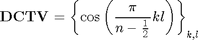
- DCTV matrix definition
- DCTV in terms of Tschebyshev polynomials
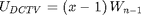
- DCTVI matrix definition
- DCTVI in terms of Tschebyshev polynomials
- Finding relations
- Check expression of DCTV through DCTVI
- Check expression of DCTVI through DCTV
- Check computation of DCTV transform
- Check computation of DCTVI transform
- Reference
Definitions
Transform matrix is defined for operating on column-vectors y=T*x, where y, x are column-vectors, T is transform matrix
DCTV matrix definition
N1=8; N=N1;
k=0:N1-1;  l=0:N1-1;
DCT5=cos(pi/(N-1/2)*k'*l)       % display DCTV matrix
DCT5 =
  Columns 1 through 7
    1.0000    1.0000    1.0000    1.0000    1.0000    1.0000    1.0000
    1.0000    0.9135    0.6691    0.3090   -0.1045   -0.5000   -0.8090
    1.0000    0.6691   -0.1045   -0.8090   -0.9781   -0.5000    0.3090
    1.0000    0.3090   -0.8090   -0.8090    0.3090    1.0000    0.3090
    1.0000   -0.1045   -0.9781    0.3090    0.9135   -0.5000   -0.8090
    1.0000   -0.5000   -0.5000    1.0000   -0.5000   -0.5000    1.0000
    1.0000   -0.8090    0.3090    0.3090   -0.8090    1.0000   -0.8090
    1.0000   -0.9781    0.9135   -0.8090    0.6691   -0.5000    0.3090
  Column 8
    1.0000
   -0.9781
    0.9135
   -0.8090
    0.6691
   -0.5000
    0.3090
   -0.1045
DCTV in terms of Tschebyshev polynomials
The DCTV matrix can be expressed in terms of Tschebyshev polynomials [1]
![$${\mathbf {DCTV}} = \left[ {T_l \left( {\alpha _k } \right)} \right]_{k,l} $$](DCTV_DCTVI_eq28569.png)
where
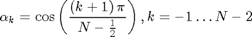
are roots of polynomial
alpha=sort([roots(TschebyshevW(N-1)); 1],'descend');
DCT5t=zeros(N1);
for l=0:N1-1,
    DCT5t(:,l+1)=polyval(TschebyshevT(l),alpha)';
end
Da5=diag(cos(0*pi/(N-1/2)*k));
DCT5t=Da5*DCT5t                    % display DCTV matrix

% compare DCT5 and DCT5t matrices (show that both definitions above are equivalent)
max(max(abs(DCT5-DCT5t)))
DCT5t =
  Columns 1 through 7
    1.0000    1.0000    1.0000    1.0000    1.0000    1.0000    1.0000
    1.0000    0.9135    0.6691    0.3090   -0.1045   -0.5000   -0.8090
    1.0000    0.6691   -0.1045   -0.8090   -0.9781   -0.5000    0.3090
    1.0000    0.3090   -0.8090   -0.8090    0.3090    1.0000    0.3090
    1.0000   -0.1045   -0.9781    0.3090    0.9135   -0.5000   -0.8090
    1.0000   -0.5000   -0.5000    1.0000   -0.5000   -0.5000    1.0000
    1.0000   -0.8090    0.3090    0.3090   -0.8090    1.0000   -0.8090
    1.0000   -0.9781    0.9135   -0.8090    0.6691   -0.5000    0.3090
  Column 8
    1.0000
   -0.9781
    0.9135
   -0.8090
    0.6691
   -0.5000
    0.3090
   -0.1045
ans =
   7.3178e-14
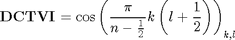
DCTVI matrix definition
N2=8; N=N2;
k=0:N2-1;  l=0:N2-1;
DCT6=cos(pi/(N-1/2)*k'*(l+1/2))       % display DCTV matrix
DCT6 =
  Columns 1 through 7
    1.0000    1.0000    1.0000    1.0000    1.0000    1.0000    1.0000
    0.9781    0.8090    0.5000    0.1045   -0.3090   -0.6691   -0.9135
    0.9135    0.3090   -0.5000   -0.9781   -0.8090   -0.1045    0.6691
    0.8090   -0.3090   -1.0000   -0.3090    0.8090    0.8090   -0.3090
    0.6691   -0.8090   -0.5000    0.9135    0.3090   -0.9781   -0.1045
    0.5000   -1.0000    0.5000    0.5000   -1.0000    0.5000    0.5000
    0.3090   -0.8090    1.0000   -0.8090    0.3090    0.3090   -0.8090
    0.1045   -0.3090    0.5000   -0.6691    0.8090   -0.9135    0.9781
  Column 8
    1.0000
   -1.0000
    1.0000
   -1.0000
    1.0000
   -1.0000
    1.0000
   -1.0000
DCTVI in terms of Tschebyshev polynomials
The DCTVI matrix can be expressed in terms of Tschebyshev polynomials [1]
![$${\bf DCTVI}={\bf D}_{DCTVI}\cdot{\left[{V_{l}\left({{\rm \beta}_{k}}\right)}\right]}_{k,l}$$](DCTV_DCTVI_eq58709.png)
where
are roots of polynomial

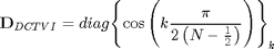
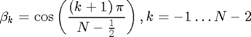
beta=sort([roots(TschebyshevW(N-1)); 1],'descend');
DCT6t=zeros(N);
for l=0:N2-1,
    DCT6t(:,l+1)=polyval(TschebyshevV(l),beta)';
end
Db6=diag(cos(1/2*pi/(N-1/2)*k));
DCT6t=Db6*DCT6t                    % display DCTV matrix

% compare DCT6 and DCT6t matrices (show that both definitions above are equivalent)
max(max(abs(DCT6-DCT6t)))
DCT6t =
  Columns 1 through 7
    1.0000    1.0000    1.0000    1.0000    1.0000    1.0000    1.0000
    0.9781    0.8090    0.5000    0.1045   -0.3090   -0.6691   -0.9135
    0.9135    0.3090   -0.5000   -0.9781   -0.8090   -0.1045    0.6691
    0.8090   -0.3090   -1.0000   -0.3090    0.8090    0.8090   -0.3090
    0.6691   -0.8090   -0.5000    0.9135    0.3090   -0.9781   -0.1045
    0.5000   -1.0000    0.5000    0.5000   -1.0000    0.5000    0.5000
    0.3090   -0.8090    1.0000   -0.8090    0.3090    0.3090   -0.8090
    0.1045   -0.3090    0.5000   -0.6691    0.8090   -0.9135    0.9781
  Column 8
    1.0000
   -1.0000
    1.0000
   -1.0000
    1.0000
   -1.0000
    1.0000
   -1.0000
ans =
   5.3957e-14
Finding relations
Because there exist relation

and

we can express DCTV through DCTVI
![$$\begin{array}{l}
{{\mathbf{DCTV}}\mathrm{{=}}{\left[{{T}_{l}\left({{\mathit{\alpha}}_{k}}\right)}\right]}_{k\mathrm{,}l}\mathrm{{=}}{\left[{{V}_{l}\left({{\mathit{\beta}}_{k}}\right)}\right]}_{k\mathrm{,}l}\mathit{\cdot}{\mathbf{B}}\mathrm{{=}}{\left({{\mathbf{D}}_{DCTVI}}\right)}^{\mathrm{{-}}{1}}\mathbf{\cdot}{\mathbf{D}}_{DCTVI}\mathit{\cdot}{\left[{{V}_{l}\left({{\mathit{\beta}}_{k}}\right)}\right]}_{k\mathrm{,}l}\mathit{\cdot}{\mathbf{B}}\mathrm{{=}}}\\
{\mathrm{{=}}{\left({{\mathbf{D}}_{DCTVI}}\right)}^{\mathrm{{-}}{1}}\mathrm{\cdot}{\mathbf{DCTVI}}\mathrm{\cdot}{\mathbf{B}}}
\end{array} $$](DCTV_DCTVI_eq65439.png)
where
![$$
{\mathbf{B}}\mathrm{{=}}\mathrm{\frac{1}{2}}\mathrm{\left[{\begin{array}{ccccc}{2}&{1}&{}&{}&{}\\{}&{1}&{\ddots}&{}&{}\\{}&{}&{\ddots}&{1}&{}\\{}&{}&{}&{1}&{1}\\{}&{}&{}&{}&{1}\end{array}}\right]}
$$](DCTV_DCTVI_eq79587.png)
B=toeplitz([0.5 zeros(1,N-1)]',[0.5         0.5 zeros(1,N-length([0.5         0.5]))]);
B(1,1)=1;
Check expression of DCTV through DCTVI

DCT5a=Da5*inv(Db6)*DCT6*B
% compare DCT5 and DCT5a matrices (show correctness of representation of DCTV through DCTVI)
max(max(abs(DCT5-DCT5a)))
DCT5a =
  Columns 1 through 7
    1.0000    1.0000    1.0000    1.0000    1.0000    1.0000    1.0000
    1.0000    0.9135    0.6691    0.3090   -0.1045   -0.5000   -0.8090
    1.0000    0.6691   -0.1045   -0.8090   -0.9781   -0.5000    0.3090
    1.0000    0.3090   -0.8090   -0.8090    0.3090    1.0000    0.3090
    1.0000   -0.1045   -0.9781    0.3090    0.9135   -0.5000   -0.8090
    1.0000   -0.5000   -0.5000    1.0000   -0.5000   -0.5000    1.0000
    1.0000   -0.8090    0.3090    0.3090   -0.8090    1.0000   -0.8090
    1.0000   -0.9781    0.9135   -0.8090    0.6691   -0.5000    0.3090
  Column 8
    1.0000
   -0.9781
    0.9135
   -0.8090
    0.6691
   -0.5000
    0.3090
   -0.1045
ans =
   4.2188e-15
Check expression of DCTVI through DCTV

DCT6a=Db6*inv(Da5)*DCT5*inv(B);
DCT6a=DCT6a(:,:)
% compare DCT6 and DCT6a matrices (show correctness of representation of DCTVI through DCTV)
max(max(abs(DCT6-DCT6a)))
DCT6a =
  Columns 1 through 7
    1.0000    1.0000    1.0000    1.0000    1.0000    1.0000    1.0000
    0.9781    0.8090    0.5000    0.1045   -0.3090   -0.6691   -0.9135
    0.9135    0.3090   -0.5000   -0.9781   -0.8090   -0.1045    0.6691
    0.8090   -0.3090   -1.0000   -0.3090    0.8090    0.8090   -0.3090
    0.6691   -0.8090   -0.5000    0.9135    0.3090   -0.9781   -0.1045
    0.5000   -1.0000    0.5000    0.5000   -1.0000    0.5000    0.5000
    0.3090   -0.8090    1.0000   -0.8090    0.3090    0.3090   -0.8090
    0.1045   -0.3090    0.5000   -0.6691    0.8090   -0.9135    0.9781
  Column 8
    1.0000
   -1.0000
    1.0000
   -1.0000
    1.0000
   -1.0000
    1.0000
   -1.0000
ans =
   8.8818e-16
Check computation of DCTV transform
x=randn(N1,1);
disp('x''=');disp(x');
y=DCT5*x;                      % true result
disp('y''=');disp(y');
y1=Da5*inv(Db6)*DCT6*B*x;            % compute DCTV using DCTVI transform
disp('y1''=');disp(y1');
x'=
  Columns 1 through 7
    0.5377    1.8339   -2.2588    0.8622    0.3188   -1.3077   -0.4336
  Column 8
    0.3426
y'=
  Columns 1 through 7
   -0.1050    1.6041    1.8244    0.6139    4.3470    1.5019   -2.4865
  Column 8
   -3.3199
y1'=
  Columns 1 through 7
   -0.1050    1.6041    1.8244    0.6139    4.3470    1.5019   -2.4865
  Column 8
   -3.3199
Check computation of DCTVI transform
x=randn(N2,1);
disp('x''=');disp(x');
y=DCT6*x;                      % true result
disp('y''=');disp(y');
y1=Db6*inv(Da5)*DCT5*inv(B)*x;            % compute DCTVI using DCTV transform
disp('y1''=');disp(y1');
x'=
  Columns 1 through 7
    3.5784    2.7694   -1.3499    3.0349    0.7254   -0.0631    0.7147
  Column 8
   -0.2050
y'=
  Columns 1 through 7
    9.2050    4.7531    1.5242    2.9712    3.6075   -0.3323   -5.5185
  Column 8
   -1.6389
y1'=
  Columns 1 through 7
    9.2050    4.7531    1.5242    2.9712    3.6075   -0.3323   -5.5185
  Column 8
   -1.6389
Reference
[1] Markus Pueschel, Jose M.F. Moura. The Algebraic Approach to the Discrete Cosine and Sine Transforms and their Fast Algorithms SIAM Journal of Computing 2003, Vol. 32, No. 5, pp. 1280-1316.