Relations between DCT_II and DST_I
Contents
Definitions
Result of transform is y=x*T, where y, x are row-vectors T is transform matrix
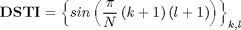
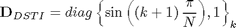
DST_I matrix definition
N=8;
DST1=sin(pi/N*((0:N-2)+1)'*((0:N-2)+1))
DST1 =
    0.3827    0.7071    0.9239    1.0000    0.9239    0.7071    0.3827
    0.7071    1.0000    0.7071    0.0000   -0.7071   -1.0000   -0.7071
    0.9239    0.7071   -0.3827   -1.0000   -0.3827    0.7071    0.9239
    1.0000    0.0000   -1.0000   -0.0000    1.0000    0.0000   -1.0000
    0.9239   -0.7071   -0.3827    1.0000   -0.3827   -0.7071    0.9239
    0.7071   -1.0000    0.7071    0.0000   -0.7071    1.0000   -0.7071
    0.3827   -0.7071    0.9239   -1.0000    0.9239   -0.7071    0.3827
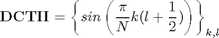
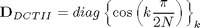
DCT_II matrix definition
DCT2=cos(pi/N*(0:N-1)'*((0:N-1)+1/2))
DCT2 =
    1.0000    1.0000    1.0000    1.0000    1.0000    1.0000    1.0000    1.0000
    0.9808    0.8315    0.5556    0.1951   -0.1951   -0.5556   -0.8315   -0.9808
    0.9239    0.3827   -0.3827   -0.9239   -0.9239   -0.3827    0.3827    0.9239
    0.8315   -0.1951   -0.9808   -0.5556    0.5556    0.9808    0.1951   -0.8315
    0.7071   -0.7071   -0.7071    0.7071    0.7071   -0.7071   -0.7071    0.7071
    0.5556   -0.9808    0.1951    0.8315   -0.8315   -0.1951    0.9808   -0.5556
    0.3827   -0.9239    0.9239   -0.3827   -0.3827    0.9239   -0.9239    0.3827
    0.1951   -0.5556    0.8315   -0.9808    0.9808   -0.8315    0.5556   -0.1951
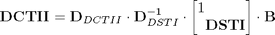
Finding relations
From [1] we know that DSTI matrix can be expressed in terms of Tschebyshev polynomials

where
are roots of polynomial
DCTII matrix can be analogously expressed as
where
are roots of polynomial

Because there exist relation

and

we can express DCTI through DSTII
where
B=-diag(ones(1,N))+diag(ones(1,N-1),-1); B(1,:)=1;
D1=diag([1, sin(pi/N*((0:N-2)+1))]);
D2=diag(cos(pi/2/N*(0:N-1)));
Check expression of DCT_II through DST_I
DST1a=eye(N);DST1a(2:end,2:end)=DST1;
D2*inv(D1)*DST1a*B
ans =
    1.0000    1.0000    1.0000    1.0000    1.0000    1.0000    1.0000    1.0000
    0.9808    0.8315    0.5556    0.1951   -0.1951   -0.5556   -0.8315   -0.9808
    0.9239    0.3827   -0.3827   -0.9239   -0.9239   -0.3827    0.3827    0.9239
    0.8315   -0.1951   -0.9808   -0.5556    0.5556    0.9808    0.1951   -0.8315
    0.7071   -0.7071   -0.7071    0.7071    0.7071   -0.7071   -0.7071    0.7071
    0.5556   -0.9808    0.1951    0.8315   -0.8315   -0.1951    0.9808   -0.5556
    0.3827   -0.9239    0.9239   -0.3827   -0.3827    0.9239   -0.9239    0.3827
    0.1951   -0.5556    0.8315   -0.9808    0.9808   -0.8315    0.5556   -0.1951
Check computation of DCTII transform
x=randn(1,N)
y=x*DCT2                           % true result
y1=x*D2*inv(D1)*DST1a*B            % compute DCTII using DSTI transform
x =
   -0.2656   -1.1878   -2.2023    0.9863   -0.5186    0.3274    0.2341    0.0215
y =
   -2.7362   -2.4709   -0.3854    0.7842    1.8413    2.7057    0.5551   -2.4187
y1 =
   -2.7362   -2.4709   -0.3854    0.7842    1.8413    2.7057    0.5551   -2.4187
Check expression of DST_I through DCT_II
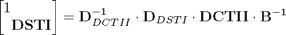
inv(D2)*D1*DCT2*inv(B)
ans =
    1.0000         0    0.0000    0.0000    0.0000    0.0000    0.0000    0.0000
    0.0000    0.3827    0.7071    0.9239    1.0000    0.9239    0.7071    0.3827
   -0.0000    0.7071    1.0000    0.7071    0.0000   -0.7071   -1.0000   -0.7071
    0.0000    0.9239    0.7071   -0.3827   -1.0000   -0.3827    0.7071    0.9239
    0.0000    1.0000    0.0000   -1.0000   -0.0000    1.0000    0.0000   -1.0000
    0.0000    0.9239   -0.7071   -0.3827    1.0000   -0.3827   -0.7071    0.9239
   -0.0000    0.7071   -1.0000    0.7071    0.0000   -0.7071    1.0000   -0.7071
   -0.0000    0.3827   -0.7071    0.9239   -1.0000    0.9239   -0.7071    0.3827
Check computation of DSTI transform
x=randn(1,N-1)
y=x*DST1                            % true result
y1=[0 x]*inv(D2)*D1*DCT2*inv(B)     % compute DSTI using DCTII transform
x =
   -1.0039   -0.9471   -0.3744   -1.1859   -1.0559    1.4725    0.0557
y =
   -2.4987   -2.6871    1.2287   -1.7412   -1.8860    2.1522   -0.8699
y1 =
   -0.0000   -2.4987   -2.6871    1.2287   -1.7412   -1.8860    2.1522   -0.8699
Reference
[1] Markus Pueschel, Jose M.F. Moura. The Algebraic Approach to the Discrete Cosine and Sine Transforms and their Fast Algorithms SIAM Journal of Computing 2003, Vol. 32, No. 5, pp. 1280-1316.