Conjugate Symmetric Sequency-Ordered Complex Hadamard Transform
Contents
Definition of CS-NCHT and CS-SCHT
CS-NCHT (Conjugate-Symmetric Natural-Ordered Hadamard Transform) is defined by next recurrence equation
![$$
{\bf H}_N = \left[ {\begin{array}{*{20}c}
{{\bf H'}_N } & {{\bf H'}_N } \\
{{\bf H'}_{N/2} {\bf S}_{N/2} } & { - {\bf H'}_{N/2} {\bf S}_{N/2} } \\
\end{array}} \right]
$$](CS_SCHT_publish_eq85015.png)
where
![$$
{\bf S}_{N/2} = \left[ {\begin{array}{*{20}c}
{{\bf I}_{N/4} } & 0 \\
0 & {j{\bf I}_{N/4} } \\
\end{array}} \right]
$$](CS_SCHT_publish_eq07170.png)
![$$
{\bf H'}_N/2 = \left[ {\begin{array}{*{20}c}
{{\bf H'}_N/4 } & {{\bf H'}_N/4 } \\
{{\bf H'}_{N/4} {\bf I'}_{N/4} } & { - {\bf H'}_{N/4} {\bf I'}_{N/4} } \\
\end{array}} \right]
$$](CS_SCHT_publish_eq80336.png)
![$$
{\bf I'}_{N/4} = \left[ {\begin{array}{*{20}c}
{{\bf I}_{N/8} } & 0 \\
0 & {-{\bf I}_{N/8} } \\
\end{array}} \right]
$$](CS_SCHT_publish_eq21306.png)
These equations correspond to Eq. (3),(4),(5),(6) from [1].
Below are presented examples of CS-NCHT transform matrices for n=2, 4, 8
for n=[2,4,8], eval(['CS_NCHT_' num2str(n) '=CS_NCHT_matrix(n),']); end
CS_NCHT_2 =
     1     1
     1    -1
CS_NCHT_4 =
   1.0000             1.0000             1.0000             1.0000
   1.0000            -1.0000             1.0000            -1.0000
   1.0000                  0 + 1.0000i  -1.0000                  0 - 1.0000i
   1.0000                  0 - 1.0000i  -1.0000                  0 + 1.0000i
CS_NCHT_8 =
  Columns 1 through 4
   1.0000             1.0000             1.0000             1.0000
   1.0000            -1.0000             1.0000            -1.0000
   1.0000                  0 + 1.0000i  -1.0000                  0 - 1.0000i
   1.0000                  0 - 1.0000i  -1.0000                  0 + 1.0000i
   1.0000             1.0000                  0 + 1.0000i        0 + 1.0000i
   1.0000            -1.0000                  0 + 1.0000i        0 - 1.0000i
   1.0000            -1.0000                  0 - 1.0000i        0 + 1.0000i
   1.0000             1.0000                  0 - 1.0000i        0 - 1.0000i
  Columns 5 through 8
   1.0000             1.0000             1.0000             1.0000
   1.0000            -1.0000             1.0000            -1.0000
   1.0000                  0 + 1.0000i  -1.0000                  0 - 1.0000i
   1.0000                  0 - 1.0000i  -1.0000                  0 + 1.0000i
  -1.0000            -1.0000                  0 - 1.0000i        0 - 1.0000i
  -1.0000             1.0000                  0 - 1.0000i        0 + 1.0000i
  -1.0000             1.0000                  0 + 1.0000i        0 - 1.0000i
  -1.0000            -1.0000                  0 + 1.0000i        0 + 1.0000i
CS-SCHT (Conjugate-Symmetric Sequency-Ordered Hadamard Transform) is a bit-reversion version of the CS-NCHT
Below are presented examples of CS-NCHT transform matrices for n=2, 4, 8
for n=[2,4,8],
    eval(['CS_NCHT_' num2str(n) '=CS_NCHT_matrix(n);']);
    eval(['CS_SCHT_' num2str(n) '=CS_NCHT_' num2str(n) '(bitrevorder(0:n-1)+1,:),']);
end
CS_SCHT_2 =
     1     1
     1    -1
CS_SCHT_4 =
   1.0000             1.0000             1.0000             1.0000
   1.0000                  0 + 1.0000i  -1.0000                  0 - 1.0000i
   1.0000            -1.0000             1.0000            -1.0000
   1.0000                  0 - 1.0000i  -1.0000                  0 + 1.0000i
CS_SCHT_8 =
  Columns 1 through 4
   1.0000             1.0000             1.0000             1.0000
   1.0000             1.0000                  0 + 1.0000i        0 + 1.0000i
   1.0000                  0 + 1.0000i  -1.0000                  0 - 1.0000i
   1.0000            -1.0000                  0 - 1.0000i        0 + 1.0000i
   1.0000            -1.0000             1.0000            -1.0000
   1.0000            -1.0000                  0 + 1.0000i        0 - 1.0000i
   1.0000                  0 - 1.0000i  -1.0000                  0 + 1.0000i
   1.0000             1.0000                  0 - 1.0000i        0 - 1.0000i
  Columns 5 through 8
   1.0000             1.0000             1.0000             1.0000
  -1.0000            -1.0000                  0 - 1.0000i        0 - 1.0000i
   1.0000                  0 + 1.0000i  -1.0000                  0 - 1.0000i
  -1.0000             1.0000                  0 + 1.0000i        0 - 1.0000i
   1.0000            -1.0000             1.0000            -1.0000
  -1.0000             1.0000                  0 - 1.0000i        0 + 1.0000i
   1.0000                  0 - 1.0000i  -1.0000                  0 + 1.0000i
  -1.0000            -1.0000                  0 + 1.0000i        0 + 1.0000i
Fast CS-SCHT algorithm
Fast algorithm of 8-point CS-NCHT can be represented in the matrix form
![$$
\begin{array}{l}
{\bf H}_8 = \left[ {\begin{array}{*{20}c}
{{\bf H}_2 } & {} & {} & {} \\
{} & {{\bf H}_2 } & {} & {} \\
{} & {} & {{\bf H}_2 } & {} \\
{} & {} & {} & {{\bf H}_2 } \\
\end{array}} \right]\left[ {\begin{array}{*{20}c}
{{\bf I}_2 } & {} & {} & {} \\
{} & {{\bf S}_2 } & {} & {} \\
{} & {} & {{\bf I}_2 } & {} \\
{} & {} & {} & {{\bf I'}_2 } \\
\end{array}} \right] \\
\bullet \left[ {\begin{array}{*{20}c}
{{\bf I}_2 } & {{\bf I}_2 } & {} & {} \\
{{\bf I}_2 } & { - {\bf I}_2 } & {} & {} \\
{} & {} & {{\bf I}_2 } & {{\bf I}_2 } \\
{} & {} & {{\bf I}_2 } & { - {\bf I}_2 } \\
\end{array}} \right]\left[ {\begin{array}{*{20}c}
{{\bf I}_4 } & {} \\
{} & {{\bf S}_4 } \\
\end{array}} \right]\left[ {\begin{array}{*{20}c}
{{\bf I}_4 } & {{\bf I}_4 } \\
{{\bf I}_4 } & { - {\bf I}_4 } \\
\end{array}} \right] \\
\end{array}
$$](CS_SCHT_publish_eq78396.png)
This equation corresponds to Eq. (34) from [1].
Signal flow graph illustrating the computation of an 8-point CS-SCHT is presented below.
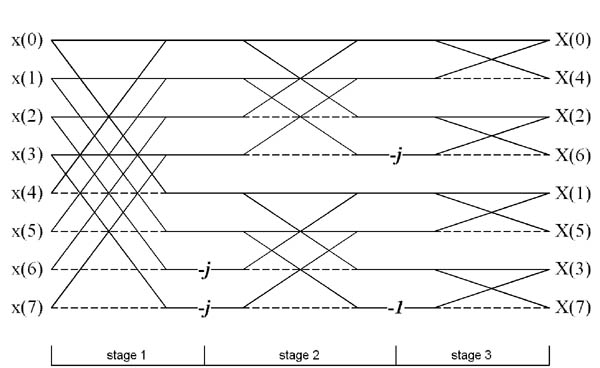
This figure corresponds to Fig. 2 from [1].
Properties of CS-SCHT transform
1. Approximation of sinusoidal waves
rCS-SCHT (real Conjugate-Symmetric Sequency-Ordered Hadamard Transform) is defined as transformation of CS-SCHT matrix using next rule
![$$
{\bf H}_{R,8} = \left[ {\begin{array}{*{20}c}
{{\bf H}_8 (0,:)} \\
{\frac{1}{2}\left( {J\left\{ {{\bf H}_8 (1,:)} \right\} - J\left\{ {{\bf H}_8 (7,:)} \right\}} \right)} \\
{\frac{1}{2}\left( {R\left\{ {{\bf H}_8 (1,:)} \right\} + R\left\{ {{\bf H}_8 (7,:)} \right\}} \right)} \\
{\frac{1}{2}\left( {J\left\{ {{\bf H}_8 (2,:)} \right\} - J\left\{ {{\bf H}_8 (6,:)} \right\}} \right)} \\
{\frac{1}{2}\left( {R\left\{ {{\bf H}_8 (2,:)} \right\} + R\left\{ {{\bf H}_8 (6,:)} \right\}} \right)} \\
{\frac{1}{2}\left( {J\left\{ {{\bf H}_8 (3,:)} \right\} - J\left\{ {{\bf H}_8 (5,:)} \right\}} \right)} \\
{\frac{1}{2}\left( {R\left\{ {{\bf H}_8 (3,:)} \right\} + R\left\{ {{\bf H}_8 (5,:)} \right\}} \right)} \\
{{\bf H}_8 (4,:)} \\
\end{array}} \right]
$$](CS_SCHT_publish_eq33672.png)
rCS-SCHT matrix has the form
rCS_SCHT_8=[CS_SCHT_8(1,:); zeros(8-2,8); CS_SCHT_8(end/2+1,:)];
rCS_SCHT_8(   2:2:end-1 ,:)=imag(CS_SCHT_8(2:end/2,:)-CS_SCHT_8(end:-1:end/2+2,:))/2;
rCS_SCHT_8(1+(2:2:end-1),:)=real(CS_SCHT_8(2:end/2,:)+CS_SCHT_8(end:-1:end/2+2,:))/2
rCS_SCHT_8 =
     1     1     1     1     1     1     1     1
     0     0     1     1     0     0    -1    -1
     1     1     0     0    -1    -1     0     0
     0     1     0    -1     0     1     0    -1
     1     0    -1     0     1     0    -1     0
     0     0    -1     1     0     0     1    -1
     1    -1     0     0    -1     1     0     0
     1    -1     1    -1     1    -1     1    -1
Rows of the rCS-SCHT transform matrix are approximation of sinusoids from DFT matrix, as can be seen on the figure below
CS_SCHT_approximation_sinusoidal_waves
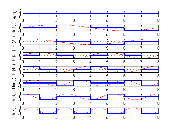
This figure corresponds to Fig. 1 of [1].
It can be checked that for dimensionality higher than 8, approximation became not good enough. This fact is reflected in spectrum figures.
2. Spectrum of CS-SCHT and FFT basis functions (case N=8)
Figures below illustrates magnitude response for each row vector of CS-SCHT and FFT matrices for n=8.
n=8;
CS_SCHT_freqresp;
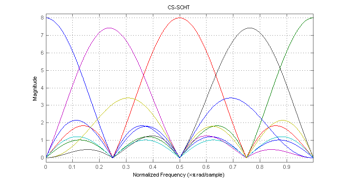
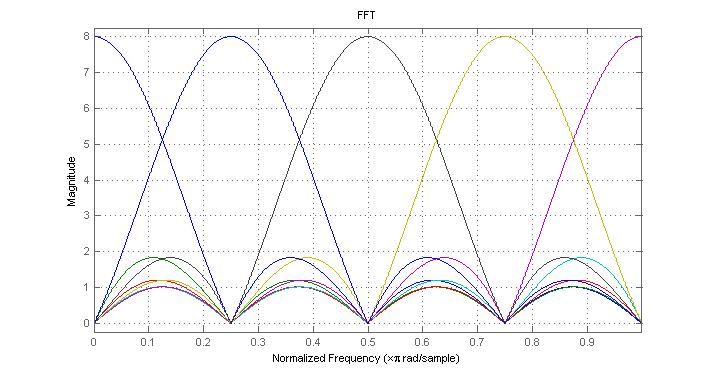
These figures correspond to Figs. 3 and 4 of [1].
For dimensionality n=8 spectrum of CS-SCHT basis functions is comparable to the spectrum of FFT basis functions.
3. Spectrum of CS-SCHT and FFT basis functions (case N=32)
Figures below illustrates magnitude response for each row vector of CS-SCHT and FFT matrices for n=32.
n=32;
CS_SCHT_freqresp;
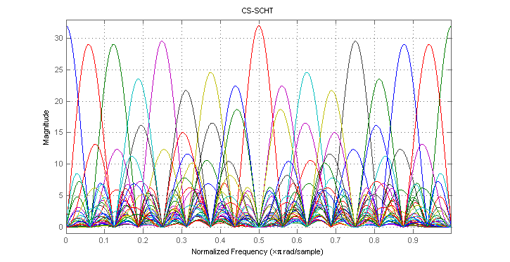
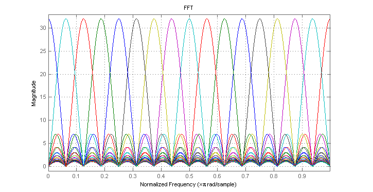
For higher dimensionality, some basis functions of CS-SCHT are spreaded considerably relative to the FFT spectrum. It makes long CS-SCHT transformation not very useful for FFT approximation. However, 8- and 16-length CS-SCHT based transforms (namely, rCS-SCHT) can be useful for image compression for example, as shown below.
Fast rCS-SCHT algorithm
Signal flow graph illustrating the computation of an 8-point real CS-SCHT is presented below.
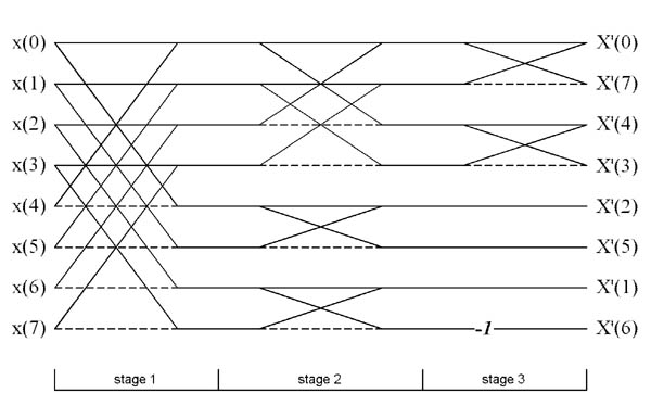
This figure corresponds to Fig. 7 from [1].
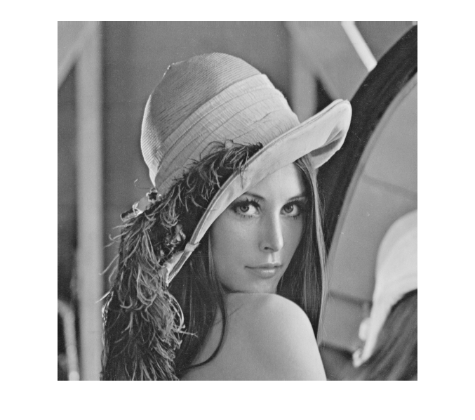
Image compression application
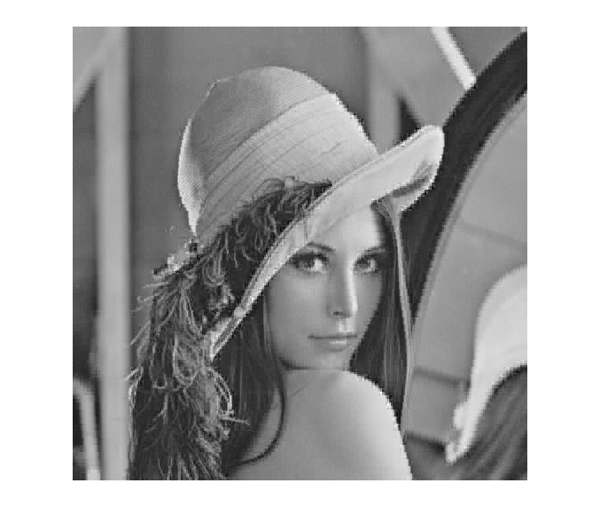
1. Visual comparison.
Using figures below it is possible visually estimate quality of image compression using DCT, HT (Hadamard Transform), and rCS-SCHT transforms. For all compressed images only 5 coefficients with maximal magnitude are remained.
Original image
a=imread('4.2.04.tiff','tiff');
a=rgb2gray(a);
imshow(a);
truesize
a=double(a);
a=a-128;
Compression using DCT
remained_coeffs=7;
b=Image_compress_DCT(a,remained_coeffs);
imshow(b,[0 255])
truesize

Compression using HT
b=Image_compress_HT(a,remained_coeffs);
imshow(b,[0 255])
truesize

Compression using CS-SCHT
b=Image_compress_CS_SCHT(a,remained_coeffs);
imshow(b,[0 255])
truesize
These figures correspond to Figs. 10(a-d) of [1].
2. MSE comparison. Here we present relations of MSE (mean square error) on the number of remained coefficients. DCT outperforms both Hadamard transform in quality by expense of highest amount of computations. On the contrary, rCS-SCHT has minimal number of arithmetical calculations and has almost the same quality as HT for majority of cases, making it attractive replacement for image compression application.
MSE comparison for 8x8 blocks
close all

load err
plot(1:length(dcterr),dcterr*8*8/sum(sum(a.^2)),'b',1:length(hterr),hterr*8*8/sum(sum(a.^2)),'g',1:length(dcshterr),dcshterr*8*8/sum(sum(a.^2)),'r')
grid on
legend('DCT','WHT','rCS-SCHT')
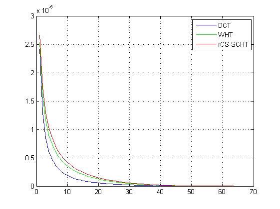
This figure corresponds to Fig. 8 of [1].
MSE comparison for 16x16 blocks
load err16
plot(1:length(dcterr),dcterr*16*16/sum(sum(a.^2)),'b',1:length(hterr),hterr*16*16/sum(sum(a.^2)),'g',1:length(dcshterr),dcshterr*16*16/sum(sum(a.^2)),'r')
grid on
legend('DCT','WHT','rCS-SCHT')
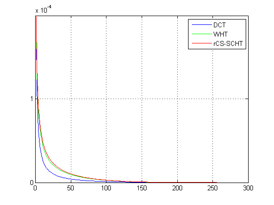
This figure corresponds to Fig. 9 of [1].
Reference
1. Aye Aung, Boon Poh Ng, Rahardja, S. Conjugate Symmetric Sequency-Ordered Complex Hadamard Transform. Signal Processing, IEEE Transactions on, July 2009, Vol. 57, N 7, pp. 2582-2593.